bayes_opt Optimizer in optimagic
This tutorial demonstrates how to use the "bayes_opt" optimizer in optimagic. To use it, you need to have bayesian-optimization package installed. You can install it with the following command:
pip install bayesian-optimization
When to use Bayesian Optimization:
Function evaluations are expensive (e.g., simulations, experiments)
The function is a black box(it cannot be expressed in closed form)
You have a limited budget of function evaluations
When gradients are unavailable or computationally expensive to obtain
Key Concepts
Gaussian Processes (GP)
The GP serves as a probabilistic model of your objective function. It provides both a mean prediction and uncertainty estimates.
Acquisition Functions
These functions use the GP’s predictions to decide where to evaluate next.
Common acquisition functions include:
Upper Confidence Bound (UCB): Balances mean prediction with uncertainty
Expected Improvement (EI): Expected improvement over the current best
Probability of Improvement (POI): Probability of improving over the current best
import numpy as np
import pandas as pd
import matplotlib.pyplot as plt

import optimagic as om
from bayes_opt import acquisition
Basic Usage of the bayes_opt Optimizer
Let’s start with a simple example using a sphere function
def sphere(params):
    return params @ params
# Note: bayes_opt requires bounds for all parameters
bounds = om.Bounds(
    lower=np.full(2, -10.0),
    upper=np.full(2, 10.0)
)
bayesopt_res = om.minimize(
    fun=sphere,
    params=np.arange(2),
    algorithm="bayes_opt",
    bounds=bounds,
    algo_options={"seed": 1}
)

bayesopt_res.params
array([-0.01729394, -0.02881131])
Acquisition Functions in the bayes_opt Optimizer
In Bayesian optimization, the acquisition function decides where to sample next. It controls the trade-off between exploration (search new areas) and exploitation (focus on good areas).
optimagic lets you set the acquisition function in different ways:
1. Using No Acquisition Function (Default)
# Uses package defaults: UCB for unconstrained, EI for constrained
acquisition_function = None
2. Using a String (Built-in acquisition functions)
You can pass any of the following strings to select a standard acquisition function:
"ucb"/"upper_confidence_bound"– Upper Confidence Bound"ei"/"expected_improvement"– Expected Improvement"poi"/"probability_of_improvement"– Probability of Improvement
acquisition_function_str = "ucb"
3. Using a Class (Auto-Instantiated)
You can also pass the class directly, optimagic will create an instance for it:
from bayes_opt.acquisition import UpperConfidenceBound

acquisition_function_class = UpperConfidenceBound
4. Using an Instance
from bayes_opt.acquisition import ExpectedImprovement

acquisition_function_instance = ExpectedImprovement(
    xi=0.1,
    exploration_decay=0.95,
    exploration_decay_delay=5
)
Example Run with configured acquisition functions
res = om.minimize(
    fun=sphere ,
    params=np.arange(2),
    algorithm="bayes_opt",
    bounds=om.Bounds(lower=np.full(2, -5.0), upper=np.full(2, 5.0)),
    algo_options={"seed":1, "acquisition_function": acquisition_function_str,}
        # acquisition_function can be any of:
        #   acquisition_function_str        → e.g. "ucb", "ei", "poi"
        #   acquisition_function_class      → e.g. UpperConfidenceBound
        #   acquisition_function_instance   → e.g. ExpectedImprovement(xi=0.1)
        #   None                            → defaults to "ucb"
    )

res.params
array([-0.01829442, -0.02171164])
Custom Acquisition Functions
bayesian-optimization also allows us to write our own acquisition functions by subclassing its AcquisitionFunction class. This allows you to define exploration/exploitation strategies tailored to your specific problem.
Implementation Requirements
When subclassing AcquisitionFunction, there are specific methods we must implement:
base_acq(self, mean, std)method (Required): This is the core method where you define the mathematical formula for your acquisition function. It takes the predicted mean and standard deviation from the Gaussian Process and returns the acquisition value(s).suggestmethod (Optional but often needed): The base class provides a default implementation, but you may need to override it if you need to set up internal state (likey_maxfor EI/PI) beforebase_acqis called.get_acquisition_paramsandset_acquisition_paramsmethods (Optional but recommended): These are used for retrieving and setting the internal parameters of your acquisition function. Implementing them makes your acquisition function fully configurable and serializable.
from bayes_opt.acquisition import AcquisitionFunction
class CustomAcquisition(AcquisitionFunction):
    """
    A simple custom acquisition function.

    This acquisition returns half of the predicted mean.
    It ignores the uncertainty (std), making it purely
    exploitation-oriented.
    """
    def __init__(self):
        super().__init__()

    def base_acq(self, mean, std):
        return 0.5 * mean
Using the Custom Acquisition Function
Once you have defined your custom acquisition function, you can use it in optimagic by passing an instance or a class to the acquisition_function parameter:
acquisition_function = CustomAcquisition()

res = om.minimize(
    fun=sphere ,
    params=np.arange(2),
    algorithm="bayes_opt",
    bounds=om.Bounds(lower=np.full(2, -5.0), upper=np.full(2, 5.0)),
    algo_options={"seed":1, "acquisition_function": acquisition_function,}
    )

res.params
array([-0.00687283, 0.0263644 ])
Meta Acquisition Functions
The bayesian-optimization package also provides meta acquisition functions that operate on other acquisition functions:
GPHedge: Dynamically chooses the best acquisition function from a set of candidates based on their past performance.
ConstantLiar: Used for parallelized optimization to discourage sampling near points that have already been suggested but not yet evaluated.
Here’s how to use GPHedge with multiple base acquisition functions:
1. GPHedge:
Dynamically chooses the best acquisition function from a set of candidates based on their past performance.
let’s define the Branin function, to use with Meta Acquisition functions.
def branin(params):
    """The Branin function - a classic optimization test function.

    Has three global minima at approximately:
    - (-π, 12.275)
    - (π, 2.275)
    - (9.42478, 2.475)

    Global minimum value: 0.397887
    """
    x1, x2 = params[0], params[1]

    a = 1
    b = 5.1 / (4 * np.pi**2)
    c = 5 / np.pi
    r = 6
    s = 10
    t = 1 / (8 * np.pi)

    term1 = a * (x2 - b * x1**2 + c * x1 - r)**2
    term2 = s * (1 - t) * np.cos(x1)
    term3 = s

    return term1 + term2 + term3
from bayes_opt.acquisition import GPHedge, UpperConfidenceBound, ExpectedImprovement

# Create a list of base acquisition functions
base_acquisitions = [
    UpperConfidenceBound(kappa=2.576),
    ExpectedImprovement(xi=0.01),
    # Add more as needed
]

gphedge_acq = GPHedge(base_acquisitions)

result = om.minimize(
    fun=branin,
    params=np.array([1.0, 1.0]),
    algorithm="bayes_opt",
    bounds=bounds,
    algo_options={
        "acquisition_function": gphedge_acq,
        "seed": 42
    }
)

result.params, result.fun
(array([9.41612935, 2.42211614]), 0.4003256667593451)
2. ConstantLiar
ConstantLiar is used for parallelized optimization. It discourages sampling near points that have already been suggested but not yet evaluated.
from bayes_opt.acquisition import ConstantLiar, UpperConfidenceBound

base_acq = UpperConfidenceBound(kappa=2.576)

constant_liar_acq = ConstantLiar(base_acquisition=base_acq, strategy="max")

# Use in optimization (Note: ConstantLiar is primarily for async optimization)
result = om.minimize(
    fun=sphere,
    params=np.array([1.0, 1.0]),
    algorithm="bayes_opt",
    bounds=bounds,
    algo_options={
        "acquisition_function": constant_liar_acq,
        "seed": 42
    }
)

result.params
array([-0.0504843 , -0.00431406])
Exploration vs Exploitation Trade-off
When using Bayesian optimization, the acquisition function decides where to sample next. It balances exploration (try new areas) vs exploitation (refine known good areas).
Exploration: Sampling in regions with high uncertainty
Exploitation: Sampling in regions with high predicted values
Related Parameters
kappa (UCB): Higher values → more exploration
xi (EI/POI): Higher values → more exploration
exploration_decay: Gradually shift from exploration to exploitation
exploration_decay_delay: When to start the decay
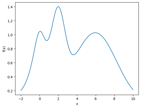
def f(x):
  """Function with multiple peaks"""
  x = x[0]
  return float(
        np.exp(-(x - 2) ** 2) +
        np.exp(-(x - 6) ** 2 / 10) +
        1 / (x ** 2 + 1)
    )
x = np.linspace(-2, 10, 100)
Y = [f([xi]) for xi in x]
plt.plot(x, Y)
plt.xlabel("x")
plt.ylabel("f(x)")
plt.show()
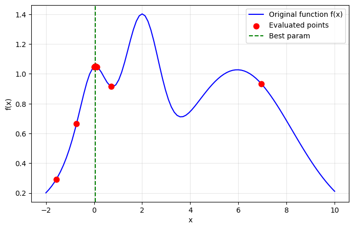
def plot_bayes_opt(result):
    """Plot optimization results"""
    evaluated_points = np.array([p[0] for p in result.history.params])
    function_values = np.array(result.history.fun)

    plt.figure(figsize=(8,5))
    plt.plot(x, Y, 'b-', label="Original function f(x)")
    plt.scatter(evaluated_points, function_values, c="red", s=60, zorder=3, label="Evaluated points")
    plt.axvline(result.params[0], color="green", linestyle="--", label="Best param")

    plt.xlabel("x")
    plt.ylabel("f(x)")
    plt.legend()
    plt.grid(True, alpha=0.3)
    plt.show()
# strategy: exploitation (kappa=0.1) - focuses on known good areas
acquisition_function = acquisition.UpperConfidenceBound(kappa=0.1)
result = om.maximize(
    fun=f,
    params=np.array([0.]),
    algorithm="bayes_opt",
    bounds=om.Bounds(lower=np.full(1, -2.0), upper=np.full(1, 10.0)),
    algo_options={
        "acquisition_function": acquisition_function,
        "seed": 987234,
    }
)

# Notice: Points cluster around peaks, might also get stuck in local optimum
plot_bayes_opt(result)
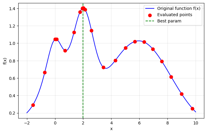
# strategy: exploration (kappa=10) - explores more broadly
acquisition_function = acquisition.UpperConfidenceBound(kappa=10)
result = om.maximize(
    fun=f,
    params=np.array([0.]),
    algorithm="bayes_opt",
    bounds=om.Bounds(lower=np.full(1, -2.0), upper=np.full(1, 10.0)),
    algo_options={
        "acquisition_function": acquisition_function,
        "seed": 987234,
    }
)

# Notice: Points are more spread out, better chance of finding global optimum
plot_bayes_opt(result)
Sequential Domain Reduction (SDR)
Sequential Domain Reduction (SDR) progressively narrows the search space around promising regions. This can significantly improve optimization, especially for high-dimensional problems.
SDR Parameters
enable_sdr: Enable/disable Sequential Domain Reductionsdr_gamma_osc: Controls oscillation damping (default: 0.7)sdr_gamma_pan: Controls panning behavior (default: 1.0)sdr_eta: Zooming parameter for region shrinking (default: 0.9)sdr_minimum_window: Minimum window size (default: 0.0)
SDR Example
def ackley(x):
    """Global minimum: f(x*) = 0 at x* = (0, 0)"""
    x0, x1 = x
    arg1 = -0.2 * np.sqrt(0.5 * (x0 ** 2 + x1 ** 2))
    arg2 = 0.5 * (np.cos(2 * np.pi * x0) + np.cos(2 * np.pi * x1))
    return -20. * np.exp(arg1) - np.exp(arg2) + 20. + np.e

start_params = np.array([2.0, 2.0])
bounds = om.Bounds(
    lower=np.array([-32.768, -32.768]),
    upper=np.array([32.768, 32.768])
)
# Standard Bayesian Optimization without SDR
result_standard = om.minimize(
    fun=ackley,
    params=start_params,
    algorithm="bayes_opt",
    bounds=bounds,
    algo_options={
        "enable_sdr": False,
        "n_iter": 50,
        "init_points": 2,
        "seed": 1,
        "acquisition_function": "ucb",
    }
)

print("Standard Bayesian Optimization:")
print("Best function value:", result_standard.fun)
print("Best parameters:", result_standard.x)
Standard Bayesian Optimization:
Best function value: 3.4319705253667157
Best parameters: [0.35175546 0.32364869]
/home/docs/checkouts/readthedocs.org/user_builds/optimagic/checkouts/632/src/optimagic/optimization/algorithm.py:310: UserWarning: The following algo_options were ignored because they are not compatible with bayes_opt:

 {'n_iter'}
  warnings.warn(msg)
# Bayesian Optimization with SDR
result_sdr = om.minimize(
    fun=ackley,
    params=start_params,
    algorithm="bayes_opt",
    bounds=bounds,
    algo_options={
        "enable_sdr": True,
        "sdr_minimum_window": 0.5,
        "sdr_gamma_osc": 0.7,
        "sdr_gamma_pan": 1.0,
        "sdr_eta": 0.9,
        "n_iter": 50,
        "init_points": 2,
        "seed": 1,
        "acquisition_function": "ucb",
    }
)

print("Bayesian Optimization with SDR:")
print("Best function value:", result_sdr.fun)
print("Best parameters:", result_sdr.x)
Bayesian Optimization with SDR:
Best function value: 1.1739338682273055
Best parameters: [0.17404486 0.03951124]
/home/docs/checkouts/readthedocs.org/user_builds/optimagic/checkouts/632/src/optimagic/optimization/algorithm.py:310: UserWarning: The following algo_options were ignored because they are not compatible with bayes_opt:

 {'n_iter'}
  warnings.warn(msg)
# Compare convergence behavior
results = {
    "Standard BO": result_standard,
    "BO with SDR": result_sdr
}

# SDR typically converges faster than standard BO
fig = om.criterion_plot(results)
fig.show()
Gaussian Process Configuration
"bayesian-optimization" uses a Gaussian Process (GP) as the surrogate model. Its behavior can be tuned with these options via algo_options:
alpha: noise level in function evaluations
lower values (e.g.,
1e-6): assumes nearly precise function evaluationshigher values (e.g.,
1e-2): assumes noisy evaluations
n_restarts: Number of times to restart the optimization.
seed → ensures reproducible results.
algo_options = {
    "alpha": 1e-3,
    "n_restarts": 5,
    "seed": 42,
}

result_configured = om.minimize(
    fun=sphere,
    params=np.array([3.0, 3.0]),
    algorithm="bayes_opt",
    bounds=om.Bounds(lower=np.full(2, -5.0), upper=np.full(2, 5.0)),
    algo_options=algo_options
)

print("Configured GP results:")
print(f"  Best value: {result_configured.fun}")
print(f"  Function evaluations: {result_configured.n_fun_evals}")
Configured GP results:
  Best value: 0.002346115576446452
  Function evaluations: 31
Summary
Bayesian optimization is a powerful tool for optimizing expensive black-box functions. Key takeaways:
Choose the right acquisition function based on your exploration/exploitation needs
Tune acquisition parameters like kappa (UCB) or xi (EI) to control the trade-off
Use SDR for high-dimensional problems to focus the search
Configure the GP properly with appropriate noise levels and restarts
For more detailed information, check out the bayesian-optimization documentation.